Image-based Workflow
Image-based_Workflow.Rmd1. Overview
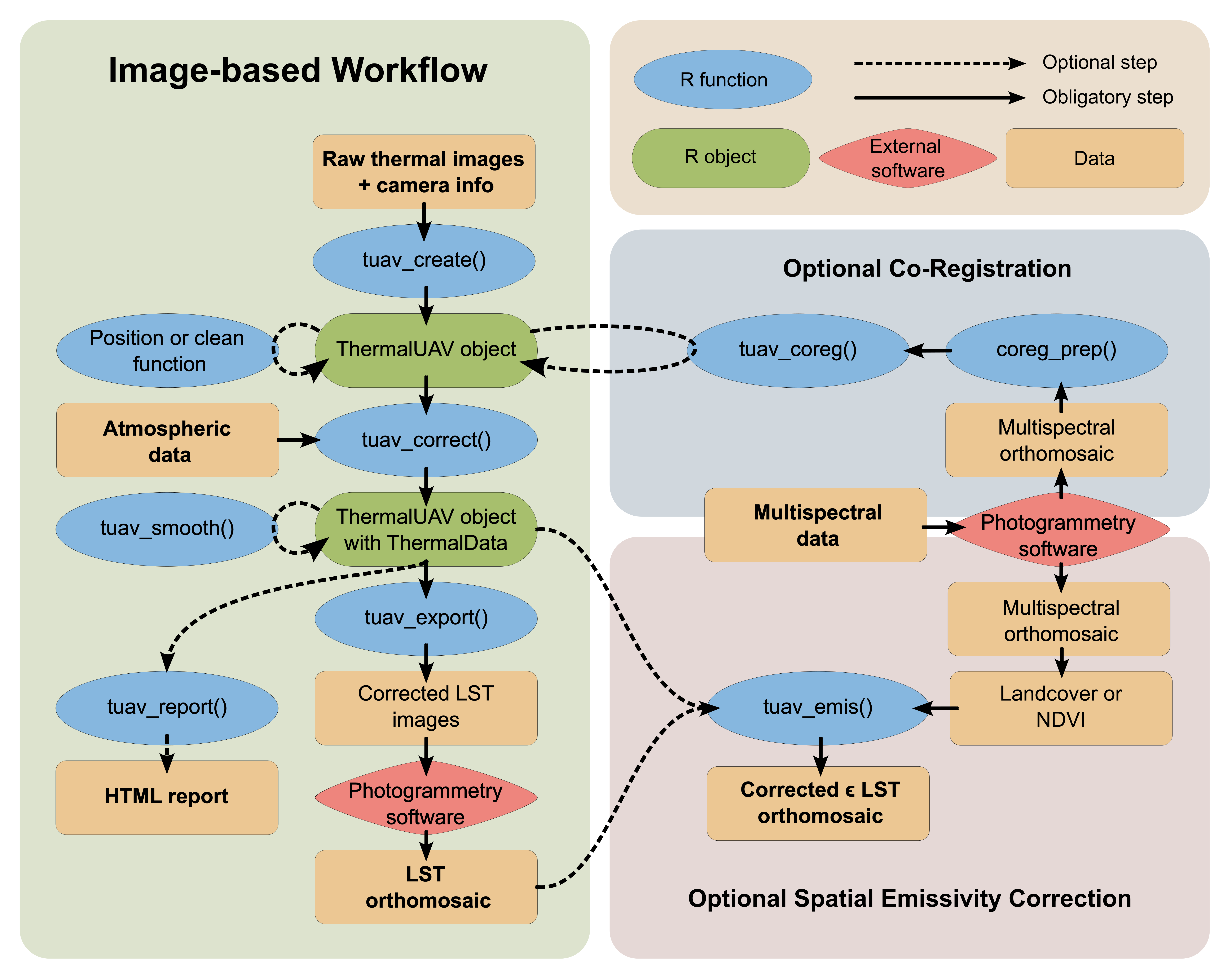
In this article we will go over the image-based workflow step by step. The image-based workflow is intended to perform corrections at image level. The following figure provides a more detailed overview of the image-based workflow, indicating additional functionalities. The different steps will be explained suing two examples:
2. Basic workflow with DJI Matrice 3T
First things first, before we start we need to load the R package in our environment:
Once this is complete we can call the functions embedded in the R package
When using DJI cameras in the image-based workflow, the package
utilizes the DJI Thermal SDK functionality provided by DJI. The package
uses a c++ function get_temp_dirp_cpp() (through Rcpp) in
the background to access the libraries provided by DJI.
2.1. Create a ThermalUAV object
The image-based workflow always starts with creating a ThermalUAV
object using the function tuav_create(). Here we will give
the name “thermal_uav” to the ThermalUAV object. The path refers to the
path on your pc to the folder containing the TIFF/jpg files, or path to
1 TIFF/jpg file. The camera name can be found by running the function
tuav_cameras(). The flight_height is our case 75 meters. No
external metadata dataframe is available so we set it to NA, this way
only the meta data stored in exif will be used.
thermal_uav <- tuav_create(path = "E:/Thermal_Project/Thermal_data_dji",
                           camera = "DJI_M3T",
                           meta_csv = NA,
                           flight_height = 75)
2.2. Conversion to LST
After creating the ThermalUAV you can already correct the data using
the function tuav_correct(). Here, atmospheric data is
required, use the expression “?tuav_correct()” to check which formats
can be used. In this example we keep it simple and will only use one
value for each atmospheric parameter, as the flight was relatively short
and was performed under stable weather conditions. The values were
measured using the portable Kestrel 5000 weather station. The parameter
flight_height is set to NA to use the height as defined in
tuav_create(). Emissivity is set to 0.985, a commonly used
value for vegetation. To obtain the background temperature
T_bg in Kelvin, the brightness temperature of crumpled
aluminium foil was used.
thermal_uav_correct <- tuav_correct(thermal_uav,
                                    flight_height = NA,   # in meters
                                    T_air = 28.7,         # in °C
                                    rel_hum = 47.2,       # in %
                                    T_bg = 282.37,        # in Kelvin
                                    emiss = 0.985)
2.3. Export and report
Now the most basic, essential correction is done, and we can export
the data to convert the images into a LST orthomosaic. To export the
data, use the function tuav_export(). Make sure you use the
most up-to-date ThermalUAV object, holding the thermal information and
latest corrections. Set export_path if you want to store
the data somewhere specific. Here we use the default ‘NA’, to create a
new folder, names “corrected”, within the original folder.
tuav_export(thermal_uav_correct,
            export_path = NA)
Optionally, if desired, you can also create an HTM-report using
tuav_report():
tuav_report(thermal_uav_correct,
            project_name = "Thermal_Project_DJI",
            flight_name = "Flight 1",
            pilot_name = "Pilot X",
            location = "Flightblock Y")
2.4. Optional Spatial Emissivity Correction
After stitching the exported corrected LST tiff files, you obtain a LST orthomosaic. This LST map assumes one emissvivty value for the whole area. If you flew over a region with a lot of different land covers, some parts might be over/under estimated due to a wrong emissivity value. For example, the thermal emissivity for bare soil, vegetation and water differ. You can account for this using the NDVI threshold method, a landcover (LC) map or directly through an emissivity map if available see vignette(“Background”) for more information. The NDVI, LC or emissvity map does not necessarily have to be taken at the same day or resolution. However, it must completely cover the LST orthomosaic.
In this example we will use the NDVI threshold method. The multispectral (MSP) data was obtained using the Micasense Altum-PT on the same day and processed in Agisoft Metashape using this workflow. The reflectance was calibrated using a 50% calibration panel. The MSP orthomosaic is first loaded to create an NDVI map. You can use the terra package to work with rasters in R.
library(terra)
# Load the MSP data as SpatRaster
MSP <- rast("E:/Thermal_Project/MSP_ortho_dji.tif")
# Create NDVI using the NIR and RED band
NDVI <- (MSP$NIR - MSP$RED)/(MSP$NIR + MSP$RED)
names(NDVI) <- "NDVI"
# Load the LST data as SpatRaster
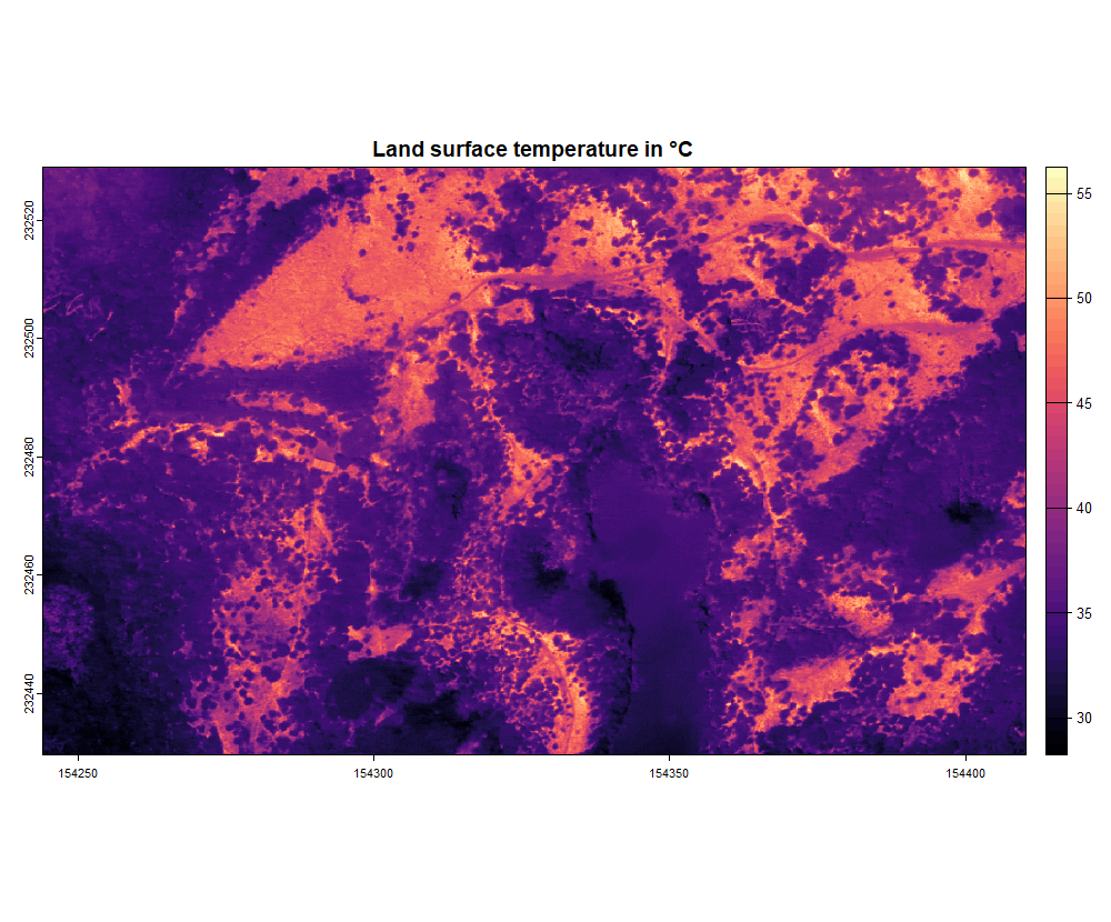
LST <- rast("E:/Thermal_Project/LST_ortho_dji.tif")
# Plot the data
par(mfrow = c(2, 1))
plot(NDVI, main = "NDVI")
plot(LST, main = "Land surface temperature in °C", col = map.pal("magma"))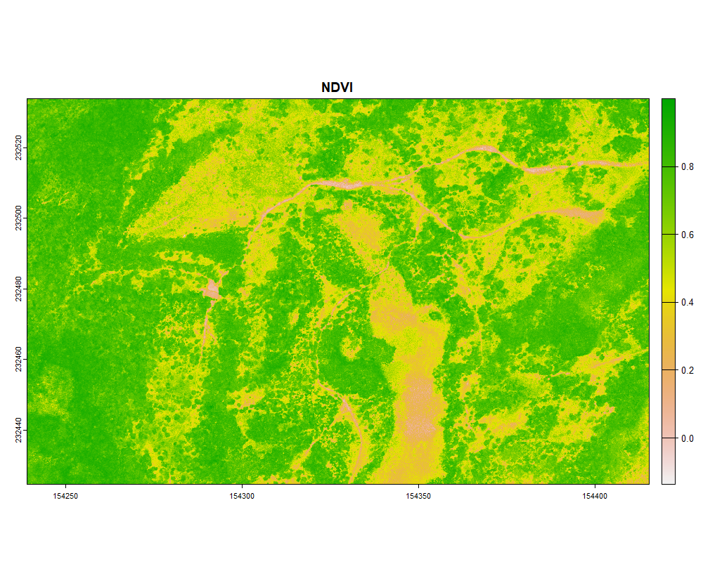
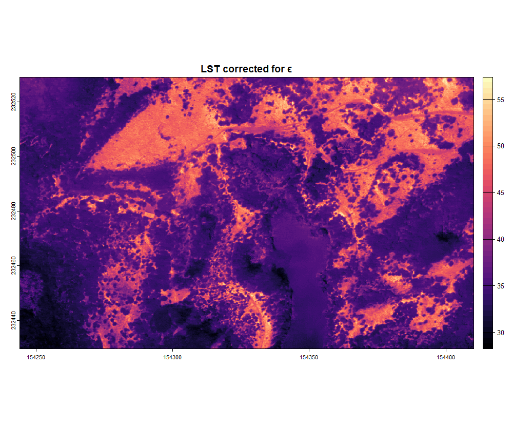
Once the NDVI map is created, we can account for the emissivity in a spatially explicit way using the NDVI threshold method. In this example we are going to set tho following parameters, the emissivity values were taken from this paper: - NDVIveg = 0.8 - NDVIsoil = 0.1 - ϵveg = 0.984 (Emissivity for shrubs) - ϵsoil = 0.914 (Emissivity for sandsoils)
LST_emis <- tuav_emis(thermal_orig = LST,
                      thermal_uav = thermal_uav_correct, # The last ThermalUAV object,
                      temp = "C", # LST is in this case in °C
                      corrmap = NDVI,
                      method = "NDVI", # Here we use the NDVI method
                      write_Ts = TRUE, # If you want to write the output
                      filename_Ts = "E:/Thermal_Project/LST_ortho_dji_emis.tif",
                      write_emiss = TRUE, # Optionally you can save the emissivity raster file
                      filename_emiss = "E:/Thermal_Project/Emis_ortho_dji.tif",
                      NDVI_veg = 0.8,
                      NDVI_soil = 0.1,
                      emiss_veg = 0.984,
                      emiss_soil = 0.914)
After correcting for the spatially explicit emissivity, the LST map is final and can be plotted or used for your analysis. Please note, in this example a small part is covered by water. The emissivity of water is slightly higher than that for shrubs. Careful interpretation of the water temperatures is thus required.
3. Advanced workflow with TeAx ThermalCapture 2.0
In this example we will dive into a more advance case using the ThermalCapture 2.0. This thermal camera records at 8.33 Hz, meaning we have slightly more than 8 thermal images per second. We will discuss how you can reduce the data volume in an efficient way, while retaining maximal quality. Furthermore, we will discuss how the co-registration works, in this case with the Micasense Altum-PT. As the flight in this example is quite long covering 17 ha, we will use atmospheric data recorded at high frequency. But, first things first, we have to create a ThermalUAV object.
3.1. Create a ThermalUAV object
As in section 2.1. Create a
ThermalUAV object we will create a ThermalUAV object using the
function tuav_create(). The ThermalCapture line from TeAx,
stores thermal data as a “.TMC” file. They provide a software called
ThermoViewer to convert the TMC files into TIFF files containing the
thermal data. This software provides the option to store the metadata of
all images in ONE csv file. This csv file can be used as additional meta
data in the tuav_create() function.
thermal_uav_teax <- tuav_create(path = "E:/Thermal_Project/Thermal_data_TeAx/",
                                camera = "ThermalCapture",
                                meta_csv = "E:/Thermal_Project/Thermal_data_TeAx/Thermal_Project_meta.csv",
                                flight_height = 75)
3.2. Check and clean the data
The data volume is quite high (16612 images) as you can see with the following code:
thermal_uav_teax@Info@dataset_length You can also check the visually where all these images are located in space using the following code:
thermal_uav_teax_loc <- tuav_loc(thermal_uav_teax,
                                 extent = TRUE,   # Calculate the image extents
                                 overlap = TRUE)  # Calculate the mean frontal overlap

thermal_uav_teax_loc@Position@overlap
tuav_view(thermal_uav_teax_loc, extent = TRUE)
If all these images need to be converted, it might require a lot of
computing power. Generally, we also don’t need around 8 images per
second, resulting in a mean frontal overlap of 98.7 %. This R package
offers two functions to deal with data reduction. Either you keep a
predefined amount of images per second using tuav_persec(),
or you set a minimal threshold for overlap or sharpness with
tuav_reduc(). You can call “?tuav_reduc” to get more
information on the function’s parameters. Here we will use the method
overlap, which means the algorithm will select images to result in a
frontal overlap of the given value (in this case 0.9 for a frontal
overlap of 90%). The algorithm will only select images with enough
quality (i.e. above the sharpness_threshold). If this latter requirement
is not met, it will take the best option below this threshold to still
ensure the minimal required overlap. In this case, it will provide a
list on which images where kept, but do not meet the required quality
checks. Lastly, you have the option to delete the images from your local
storage (be careful with this option), or you can just move the images
to a different folder (= DEFAULT).
thermal_uav_teax_clean <- tuav_reduc(thermal_uav_teax_loc,
                                     method = "Overlap",
                                     min_overlap = 0.9,
                                     sharpness_threshold = 0.05,
                                     remove = FALSE)
You can see that the mean frontal overlap is reduced and visualize it with the interactive map:
thermal_uav_teax_clean@Position@overlap
tuav_view(thermal_uav_teax_clean, extent = TRUE)
3.3. Co-regsitration with Micasense Altum-PT
The ThermalCapture 2.0 is a standalone camera with its own GPS and power supply (does not get information from the UAV). In our sensor-platform configuration it is used together with the Micasense Altum-PT, which receives RTK GPS signals from our UAV (DJI Matrice 300 RTK). The ThermalCapture’s GPS information is only used to derive accurate timestamps. Subsequently, the accurate timestamps can then be used to retrieve the corresponding RTK GPS signal from the Micasense Altum-PT through interpolation. The co-registration has two options: - Directy: use the GPS and orientation data from the co-registered camera directly - Indirectly: First, align the cameras from the co-registered camera in Agisoft Metashape, export the optimized camera locations as csv file and these optimized GPS and orientation data.
In Both cases we first need to call the coreg_prep() to
prepare the data in the right format:
opt_cameras <- coreg_prep(img_path = "E:/Thermal_Project/data_Micasense/",
                          SfM_option = "Agisoft Metashape",
                          opt_camera_path = "E:/Thermal_Project/Reference_Cameras_Thermal_Project.txt",
                          camera_name = "Altum-PT_MSP",
                          label = "_2",
                          timezone = "UTC")
This should have returned a data.frame with 9 variables. We can now
use this in the tuav_coreg() function.
thermal_uav_teax_coreg <- tuav_coreg(thermal_uav_teax_clean,
                                     opt_cameras = opt_cameras,
                                     rig_offset = c(0, 0, 0, 0, 0, 0),
                                     timediff = 0)
Optionally you can call the tuav_view() function again
on the latest ThermalUAV object to check if the camera locations are
still places correctly (serves as quick visual check).
3.4. Conversion to LST
If you are satisfied with the performed corrections, we can now move
to the conversion of the brightness temperature to LST. Note, the
cleaning functions can also be performed after this step, but it will
require much longer computation time. As explained in 2.2. Conversion to LST, we use the
function tuav_correct() to perform the conversion.
During this rather long flight, weather variables were collected
simultaneous at a 5-second interval rate using the Kestrel 5500. This
data first needs to be loaded an put into the right format. you can
chekc the structure using the str() function. Datetime, can
be easily converted to POSIXct using as.POSIXct().
Kestrel <- read.csv("E:/Thermal_Project/Weather_data/Kestrel_tair_relhum.csv")
str(Kestrel)      # datetime is as character -> convert to POSIXct
Kestrel$datetime <- as.POSIXct(Kestrel$datetime, tz = "UTC")
After obtaining the data.frame in the right format, it can be used in
the tuav_correct() function
thermal_uav_teax_correct <- tuav_correct(thermal_uav_teax_coreg,
                                    flight_height = NA,   # in meters
                                    T_air = Kestrel,      # data.frame in °C
                                    rel_hum = Kestrel,    # data.frame in %
                                    T_bg = 268.26,        # in Kelvin
                                    emiss = 0.985)
3.5. Smooth
Optionally an additional smoothing procedure can be applied to avoid the influence of large fluctuations in T_air on the dataset. This smoothing correction is based on the following formula from this paper:
\[ \begin{align*} T_{S_{smooth}} = T_{s} - T_{air} + T_{air_{mean}} \end{align*} \]
thermal_uav_teax_smooth <- tuav_smooth(thermal_uav_teax_correct,
                                    method = "T_air")
3.6. Export and report
Now we are back at the point where we need to export the images and process them in an external photogrammetry software like Agisoft Metashape. Check section 2.3. Export and report for more details.
tuav_export(thermal_uav_teax_smooth,
            export_path = NA)
Optionally, if desired, you can also create an HTM-report using
tuav_report():
tuav_report(thermal_uav_teax_smooth,
            project_name = "Thermal_Project_TeAx",
            flight_name = "Flight 1",
            pilot_name = "Pilot X",
            location = "Flightblock Y")
3.7. Optional Spatial Emissivity Correction
In section 2.4. Optional Spatial Emissivity Correction we already discussed the option to account for spatially explicit post-processing emissivity correction. In the previous example we used the NDVI threshold method. In this case we will show the landcover option. This option requires:
- Landcover map (LC)
- Two column matrix containing the landcover labels with their corresponding emissivity values
In the example below, a LC map is provided with 5 classes as shown in the table below:
| Label | Class | Emissivity |
|---|---|---|
| 1 | Shrubs/green low vegetation | 0.984 |
| 2 | Dry vegetation/mosses | 0.962 |
| 3 | Trees | 0.983 |
| 4 | Sandy bare soil | 0.914 |
| 5 | Water | 0.991 |
The emissivity values were taken from Salisbury and D’Aria (1994) and Rubio, E., et al. (1997). First we will load the LC map and create the two-column matrix containing the labels with their corresponding emissivity value.
# Load the LC map as SpatRaster
LC <- rast("E:/Thermal_Project/LC_TeAx.tif")
# Create two-column matrix
matrix <- matrix(c(1,2,3,4,5,0.984,0.962,0.983, 0.914,0.991), ncol = 2)
# Load the LST data as SpatRaster
LST_teax <- rast("E:/Thermal_Project/LST_TeAx.tif")
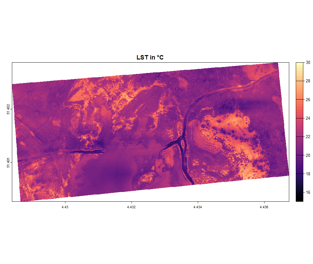
# Plot the data
par(mfrow = c(2, 1))
plot(LC, main = "Landcover", type = "classes", levels = c("Shrubs", "Mosses", "Trees", "Sandy soil", "Water"), legend = "topleft")
plot(LST_teax, main = "LST in °C", col = map.pal("magma"), range = c(15,30))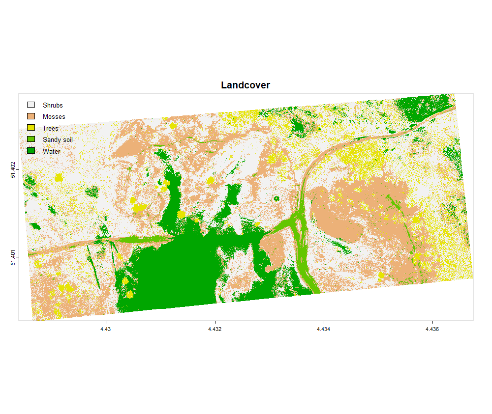
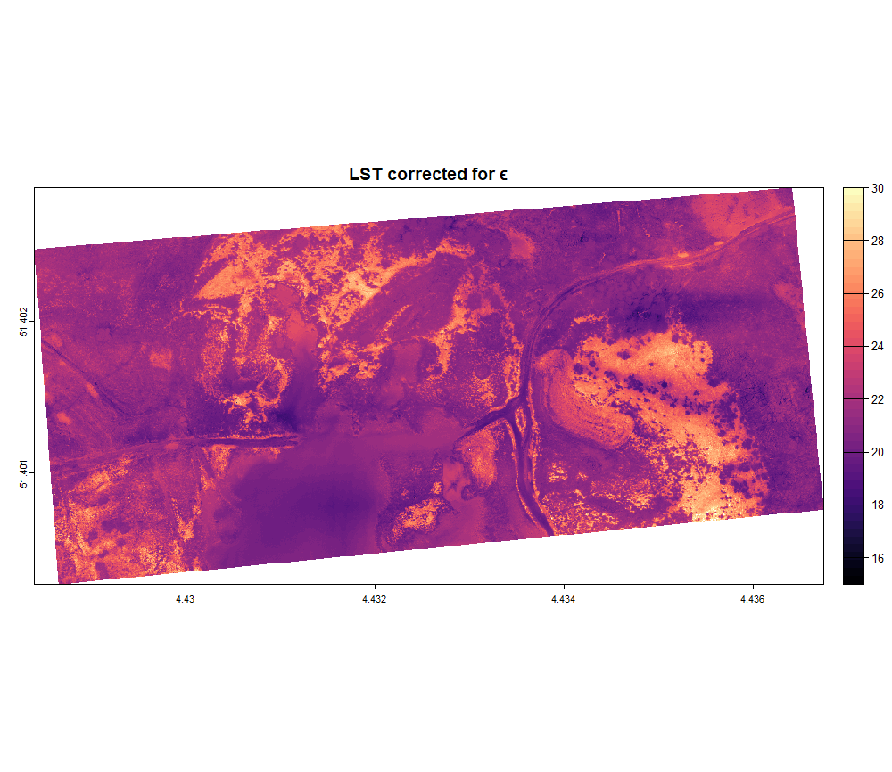
LST_teax_emis <- tuav_emis(thermal_orig = LST_teax,
                      thermal_uav = thermal_uav_teax_smooth, # The last ThermalUAV object,
                      temp = "C", # LST is in this case in °C
                      corrmap = LC,
                      method = "LC", # Here we use the LC method
                      write_Ts = TRUE, # If you want to write the output
                      filename_Ts = "E:/Thermal_Project/LST_TeAx_emis.tif",
                      write_emiss = TRUE, # Optionally you can save the emissivity raster file
                      filename_emiss = "E:/Thermal_Project/Emis_ortho_TeAx.tif",
                      LC_emiss_matrix = matrix)
After correcting for the spatially explicit emissivity, the LST map is final and can be plotted or used for your analysis.
References
- Salisbury, J.W. and D’Aria, D.M. (1994) ‘Emissivity of terrestrial materials in the 3-5 μm atmospheric window’, Remote Sensing of Environment, 47(3), pp. 345–361. Available at: https://doi.org/10.1016/0034-4257(94)90102-3.
- Rubio, E., Caselles, V. and Badenas, C. (1997) ‘Emissivity Measurements of Several Soils and Vegetation Types in the 8-14/ m Wave Band: Analysis of Two Field Methods’, Remote Sensing of Environment, 59(3), pp. 490-521. Available at: https://doi.org/10.1016/S0034-4257(96)00123-X